Reproducible analysis: orchestration
This post will cover the handling complexity part as outlined in the introduction post of this series. Originally I was aiming to use make, just as in the original series of posts which inspired mine. After some consideration I chose to opt for Airflow:
- it’s used heavily at work
- I have no experience at all using it (in contrast with
makewhich I used in a basic way from time to time) - it comes with out-of-the-box integrations
- leverages Python abilities
All of the above should make the learning curve of Airflow lower than the make learning curve. make on the other hand is more portable (since it’s not based on any high-level programming language like Python).
Issue
In the previous post of this series we wrote the functions needed for each part of the analysis. In the literate programming post we weaved together these functions with the analysis text. However, this is not a really flexible format. Say for example we just want to experiment a bit with the input data and see how this affects the models or plots afterwards? Updating the RMarkdown report for each experiment is very unwieldy.
There are two approaches we can take to make running the analysis more flexible. Both of them involve running code through the command line.
- we can parametrize the report
- we can create separate scripts combining several functions together
Parametrizing reports
Parametrizing means we can run the report with different input values. You define the parameters you want to use at the top of the report and have access to them within your report. By running the rmarkdown render command you can pass the exact values to use to the report.
I chose not to go this way because it’s still not flexible enough. It’s true you can change the inputs but the order in which functions are called remains fixed.
Separate scripts
The second approach is to:
- create scripts combining all the functions for a logical phase in the analysis
- make these scripts executable from the command line
- run these scripts in a orchestrator (e.g.
Airflow)
Advantage here is we can combine these script in any order we want, let them depend on eachother however we want,… Since this is the most flexible way, this is the path I chose to take.
Creating scripts
Scripts are in essence just a combination of functions who logically belong together. Since the creating scripts and running them from the command line steps are so tightly interwoven, I discuss them together in this part. Take as an example the transform script:
#!/usr/bin/env Rscript
library(magrittr)
library(reproseries)
library(readr)
library(docopt)

'Usage:
transform-script.R <input_path> <output_path>

]' -> doc

arguments <- docopt(doc)

readr::read_csv(file = arguments$input_path) %>%
  reproseries::addCelsiusColumn() %>%
  reproseries::summariseAvgTemperatureByYear() %>%
  readr::write_csv(path = arguments$output_path)
Each of these scripts has roughly the same structure:
- shebang at the top
- loading of libraries used
- a
docoptdescription - the functions themselves
The shebang #!/usr/bin/env Rscript says to run our script using Rscript. Alternatives to Rscript exist like R CMD BATCH. Since Rscript did the job for me I decided just to stick with it. To really be able to execute the script from the command line you have to make sure it’s executable by running chmod +x {file}.
The libraries loaded contain of course our main package reproseries but also additional helper libraries like magrittr for its pipe operator, readr to easily deal with reading and writing to disk and docopt which helps in parametrizing the script. docopt can do way more than just parametrizing but the parametrization was all I needed for Airflow.
In the code itself I first read an input data csv, run the functions related to transforming found at R/transform.R and then write the transformed data to file. In the usage part you can see both <input_path> and <output_path> are specified. Because these are written between angel brackets docopt interprets them as command arguments. This means they are mandatory. I want the input and output paths to be flexible so later on I can orchestrate them to be written anywhere I want (might be locally, might be in the cloud).
Run scripts with Airflow
What is a DAG?
We have abstracted our functions together into several logical scripts which we can run from the command line. This is where Airflow comes into play. Airflow helps you in managing tasks and their dependencies. The main concept to grasp about Airflow is the DAG. DAG is a mathemical term meaning Directed Acyclic Graph. It sounds complex but its meaning is easy to deviate:
- it’s a graph because it consists of nodes and connections between those nodes
- it’s directed because the connections have a direction
- it’s acyclic because the directions are one-way
In Airflow speak the nodes are tasks and the connection between nodes are dependencies. Once a task is done there’s no way to go back to that task in the same run.
The DAG is the most important concept but just a DAG won’t get us far. The DAG just defines in what order the work has to be done, the work itself is done in operators and tasks. Let’s have a look at the DAG used for the analysis of the temperatures. There are several parts in this file:
- importing the libraries needed
- the DAG definition
- the tasks based on operators
- a definition of the dependencies
DAG definition
Defining the DAG is very easy:
dag = DAG(dag_id='temperatures',
          start_date=datetime(2019, 1, 1))
Main thing here is the DAG has an id so it can be used as a namespace of tasks.
Tasks and operators
I created a script for each analysis phase (tidy, transform, visualize and model) and each script/analysis phase also corresponds with a task. All tasks look more or less like this:
tidy = BashOperator(
    task_id='tidy',
    bash_command=f'{os.getcwd()}/exec/tidy-script.R {os.getcwd()}/data/tidy-temperatures.csv',
    dag=dag)
An operator is the template for the task. Tasks are closely related to operators. Just as classes in object-oriented programming are templates which can be instantiated, so operators are templates which can be instantiated. An instantiated operator is called a task. In this case the task is tidy.
There was no real alternative to using the BashOperator. At some time work was done on an operator specific to R but the work seems to have stalled since the PR containing the changes was never merged in the main Airflow branch.
We use the getcwd method from the os module as to be able to run the DAG in different environments. The bash command always expects an absolute path although I couldn’t find this documented anywhere. Experiments with relative paths didn’t pan out.
Defining the dependencies
Dependencies are defined as:
clean >> tidy >> transform >> [visualize, model]
Dependencies can be configured either by using the set_upstream and set_downstream functions or by using the bit shift operators >> and <<. The bit shift operators are more readable. Note as well this doesn’t mean you can’t define the same dependency for multiple tasks at once. You can do this by using brackets.
Running the DAG
Following the instructions in the reproseries README it’s very easy to run the analysis with Airflow:
airflow backfill temperatures -s 2019-01-01
I do not use the start date but when it’s not specified Airflow throws an exception asking to provide at least a start date. In the backfill documentation however it’s not a mandatory argument. You can specify any date as start date as long as it’s a date in the past.
When you run the command above you get all the results in the terminal. Airflow also provides a UI which helps in seeing what tasks are in progress or debugging with logs if something went wrong. There’s no need to configure this UI and it provides a lot out of the box. The graph view for example shows how the tasks are related and the result for each task in the last run.
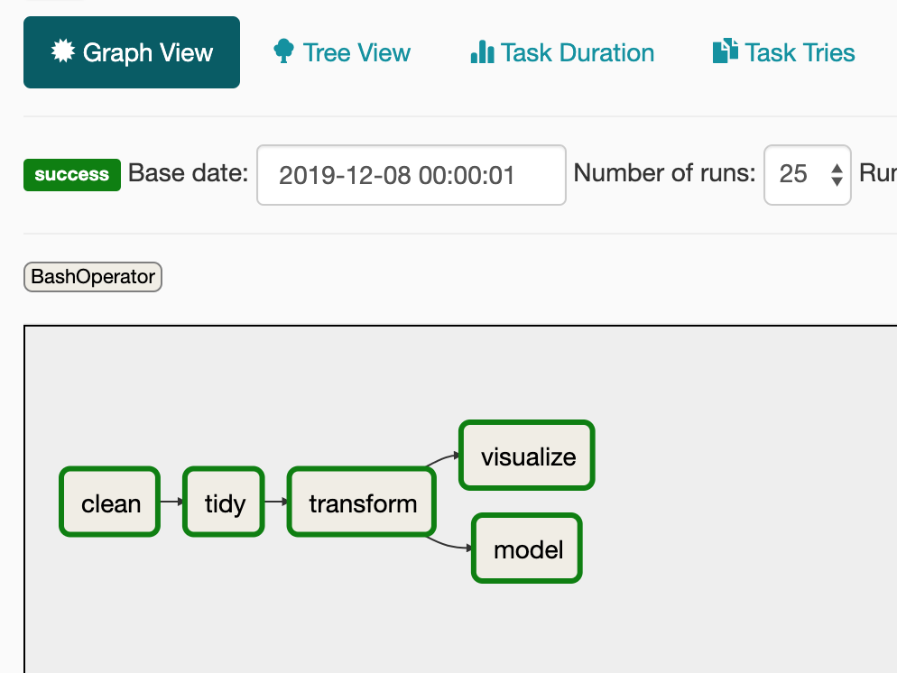
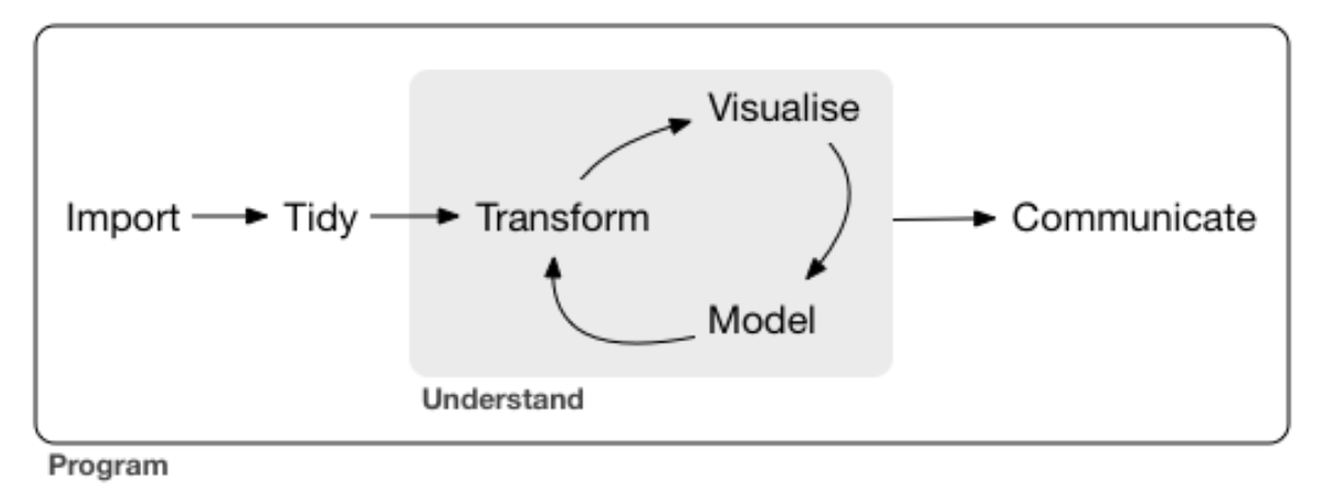
This is almost a literal mapping of the theoretical framework applied from the R for Data Science book.
The clean job is added just to make sure previously saved data is removed before starting the next run.
Having easy access to the logs is also handy to see what exactly went wrong:
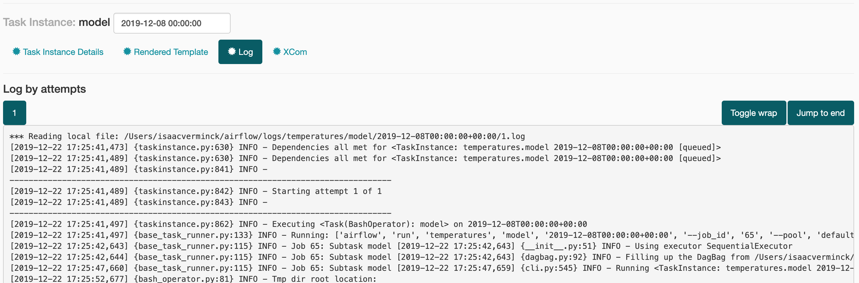
Other views are available to see runs by status (succesful, failed , queued, …), see how long each task took,…
Summary
I just scratched the Airflow surface in this post. There’s way more. We could for example experiment with the input data and see how it changes the model result. The above should however provide a solid foundation.
Code for this post can as usual be found in the reproseries repository. The README contains an Airflow part detailing how to do the setup, how to run airflow, how to get access to the webserver,…